Nowadays, everybody rests on GPS, and nobody is capable of reading a map anymore.
Good old forest plot maps, drawn with compasses and distances measured on the ground? Gone. Trees are mapped by GPS, with variable precision and success. And there is no way anybody is capable of giving you directions on the road. You got a GPS? Use it, for Hermes’ sake.

But this post is not and old man’s rant about technology.
I’m not talking about Global Positioning System.
I’m thinking of Grant Proposal Selection.

As everybody knows, the way grant proposals are chosen for funding is a lottery (when your favourite proposal is turned down) or a very meritocratic process carried out by clever, competent reviewers (when you get funded).

Yet, it must be either one or the other, or a mix of the two.
So, while I was submitting my last grant proposal, I wondered: is this all worth the effort? What’s the point of all the energy, stress, nights up moving a sentence there, changing a word here, days on the phone discussing with collaborators, if it all boils down to random outcome?
When success rates are very low, one may suspect that all the money spent by funding agencies to rank all those very good proposals is a waste: at the end, who’s in and who’s out may just be a matter of a fluke in the review process. Maybe one reviewer has had a bad night yesterday, so today he’s upset and will turn a mark down a notch, and out goes your great idea. It would be better to draw tickets from a lottery.

How can one check whether this is true, or not? To know whether the real good proposals are really the ones that have been funded, one should know beforehand which are the good ones. But this is tantamount to evaluating the proposals, which brings us back to square one.

There is a way to assess the process, though: playing games. I mean: doing some modelling.

So I set out and built a simple model, mimicking the French ANR’s selection process, which proceeds in two steps: a selection on short pre-proposal, followed by a second round of selection on full proposals which have passed the first check.
According to the data provided by the agency, in 2017 about 3500 proposals, out of about 7000, passed the pre-proposal phase, and an the end about 900 were funded, for a success rate of about 12-13%.

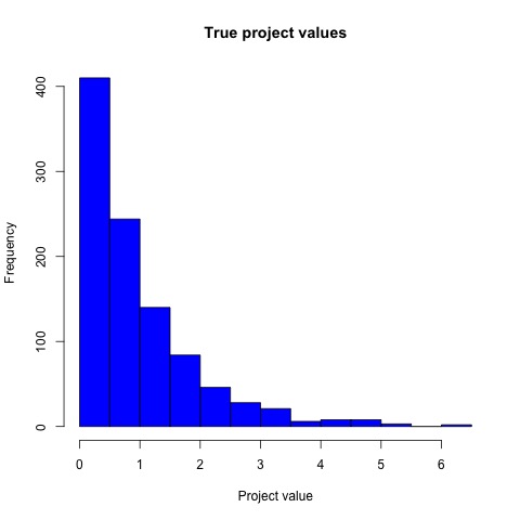
So I simulated “true” scores for 1000 “proposals” according to a gamma distribution.

The distribution of proposal true values looks like this:

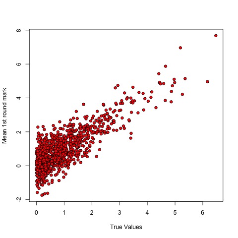
Then I supposed that two reviewers examined the proposals, each providing a score that was built by summing the true value to an “error” drawn from a gaussian with mean zero – basically, each reviewer introduced “white noise” in the score. The final pre-proposal score was the mean of the two reviewers’ scores. True to the fact that I introduced noise, the scores were dispersed around the true values.

The top half of the ranking (on the y axis, the reviewers’ scores) went on to phase two, and then the process was started all over, with a smaller error (full proposals provide more details, so it should be easier to assess their “true” value). The top 20% tier was “funded”. Then I compared the “true” scores of the winners with the final reviewers’ scores. In a perfect world, the successful proposals should be those with the best “true” values. Is this the case?

Yes and no.
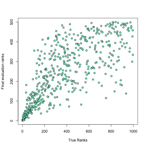
Dispersal of ranks looked large: the relationship between “true” ranking of a given proposal (x axis) and its final ranking (y axis) did not look so precise, even though there was a clear trend in favour of the best proposals:

How many of the proposals belonging to the top 20% post-evaluation are also in the top 20% of the “true” values? Around 70%.

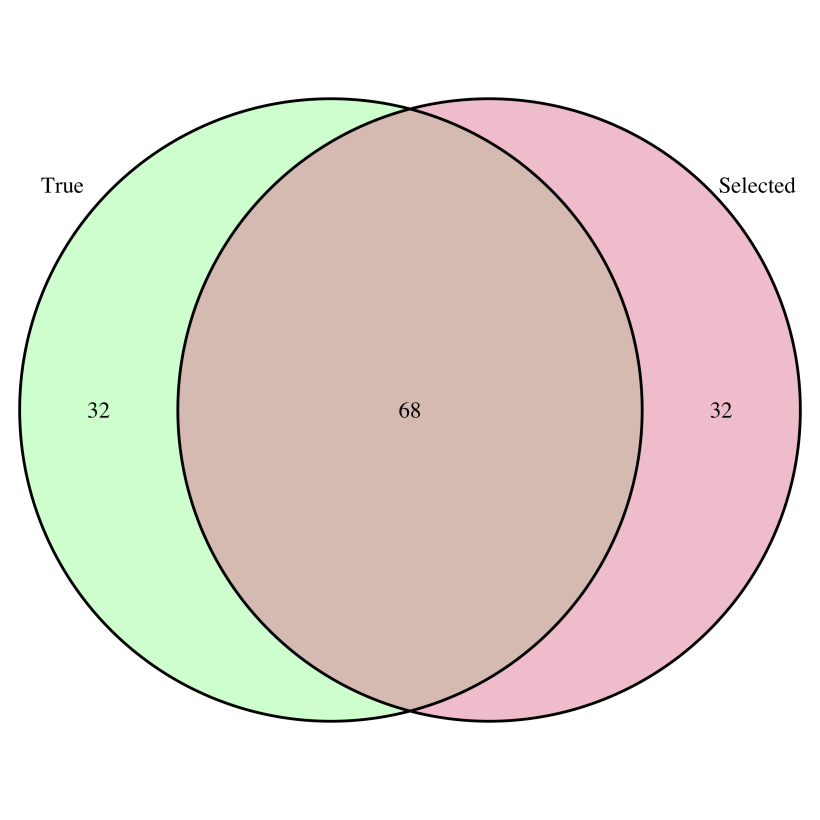
In other terms, approximately one third of the proposals that should have been selected have been turned down, and have been replaced by proposals that do not belong there. Is it satisfactory? Unsatisfactory? I’ll let you decide.
What is the alternative (apart from suppressing altogether this system for funding science)? Let us suppose that we skip the second round of selection, and that we randomly draw proposals to fund  from the proposals that have passed phase one. How do we fare?

Quite poorly. Only 16% of the funded projects are “good” ones. So, after all, there seems to be some value in the GPS (even though it can be as imprecise as a GPS under thick forest cover).

Of course, the outcome depends on the size of the error introduced by the evaluation process: increase it, and the funded projects will belong less and less to the group of the “good” ones. And I am not counting for the effect of PI previous record, nor for the fact that, if you have been funded previously, there are high chances that you’ll be funded again. Actually, a recent study – that I warmly recommend you to read – shows that, when the funding system has such a “memory”, it produces large inequality and favours luck over merit!

The R code I used to run the simulations is posted below. You can play around with it and se what happens. Enjoy the game playing – if you are not busy with a GPS.

——————–

#rule of the game:
#overall funding rate is 10%
#we start with 1000 projects.
#at first round, 50% of the proposals are selected
#at second round, 20% of the remaining projects are
#selected for funding.
#Project “true” values are gamma-distributed.
#At each step, the reviewers’ evaluation equals
#the “true” value of each project plus a white (gaussian) noise
#noise is twice as strong in the first round as in the second
#
#generating distributions of “true” project marks
nSubmitted = 1000
excludedFirstRound = 0.5
funded = 0.1
marks.gamma<-rgamma(nSubmitted,shape = 1)
#plotting:
jpeg(filename = “histTrueValues.jpg”)
hist(marks.gamma, breaks = 20, main = “True project values”,
xlab = “Project value”, col = “blue”)
dev.off()
#
#generating first round evaluator’s marks (by introducing noise)
evaluator1.noise<-marks.gamma+rnorm(n=nSubmitted, sd = 2)
evaluator2.noise<-marks.gamma+rnorm(n=nSubmitted, sd = 2)
#producing final marks (mean of two reviewers)
evalMean.noise<-rowMeans(cbind(evaluator1.noise,evaluator2.noise))
#visualising relationship:
#plotting:
jpeg(filename = “TrueValVsEvalMean.jpg”)
plot(evalMean.noise~marks.gamma,
xlab = “True Values”,
ylab = “Mean 1st round mark”,
pch = 21, bg = “red”)
dev.off()
#building a data frame
projects.df<-data.frame(seq(1,nSubmitted,1),marks.gamma,evalMean.noise)
names(projects.df)<-c(“projId”,”trueVal”,”score1stRound”)
#1st round of selection:
excluded1round<-which(projects.df$score1stRound<=quantile(projects.df$score1stRound,
probs = excludedFirstRound))
#generating 2nd round scores:
evaluator1.noise<-marks.gamma+rnorm(n=nSubmitted,sd = 1)
evaluator2.noise<-marks.gamma+rnorm(n=nSubmitted,sd = 1)
evalMean.noise<-rowMeans(cbind(evaluator1.noise,evaluator2.noise))
projects.df$score2ndRound<-evalMean.noise
projects.df$score2ndRound[excluded1round]<-NA
#computing ranks:
projects.df$trueRanking<-rank(-projects.df$trueVal)
projects.df$ranking2ndRound<-rank(-projects.df$score2ndRound)
projects.df$ranking2ndRound[excluded1round]<-NA

#let us have a look at the rankings based on true scores vs final rankings:
#plotting:
jpeg(filename = “rankVsRank.jpg”)
plot(projects.df$ranking2ndRound~projects.df$trueRanking,
xlab = “True Ranks”,
ylab = “Final evaluation ranks”,
pch = 21, bg = “aquamarine”)
dev.off()
#
projectsFunded.df<-projects.df[which(projects.df$ranking2ndRound<=nSubmitted*funded),]
projectsRandomlyFunded.df<-projects.df[sample(
which(is.na(projects.df$ranking2ndRound)==F), size = nSubmitted*funded),]
projectsBestTrueRanks.df<-projects.df[which(projects.df$trueRanking<=nSubmitted*funded),]
#how effective is the selection process?
length(intersect(projectsBestTrueRanks.df$projId,projectsFunded.df$projId))
length(intersect(projectsBestTrueRanks.df$projId,projectsRandomlyFunded.df$projId))
library(VennDiagram)
#plotting
venn.diagram(list(True = projectsBestTrueRanks.df$projId,
Selected = projectsFunded.df$projId),
filename = “selection.png”,
imagetype = “png”,
fill=c(“palegreen”,”palevioletred”))
#
venn.diagram(list(True = projectsBestTrueRanks.df$projId,
Random = projectsRandomlyFunded.df$projId),
filename = “random.png”,
imagetype = “png”,
fill=c(“palegreen”,”sandybrown”))
#